Waterfall charts, also known as bridge charts, are powerful tools for visualizing how an initial value is affected by a series of positive and negative changes, ultimately leading to a final value. They are particularly useful for financial reporting, such as illustrating net income by breaking down revenue and expenses. This guide will walk you through creating and customizing these charts in Microsoft Excel.
Understanding Waterfall Charts
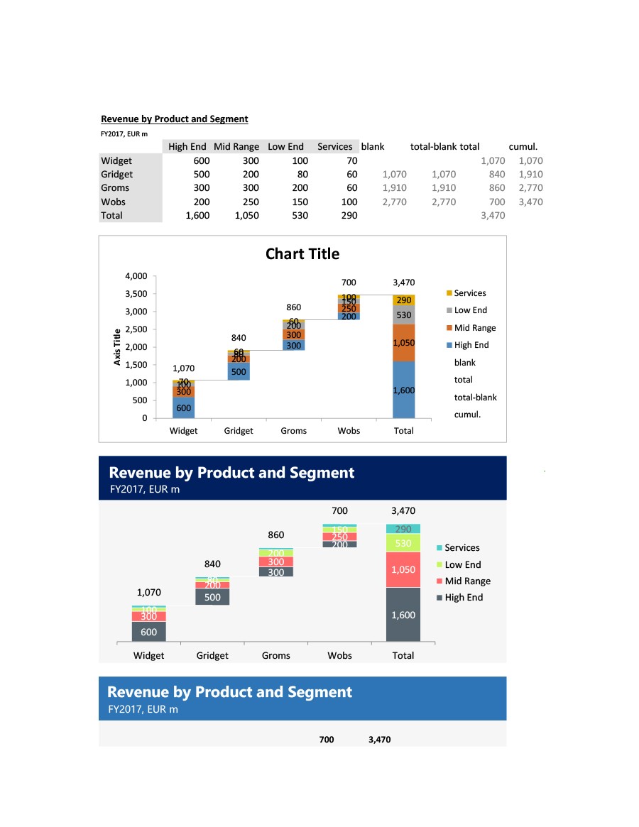
A waterfall chart displays a running total as values are added or subtracted. The columns are color-coded to easily distinguish between positive and negative contributions. Typically, the initial and final value columns are anchored to the horizontal axis, while intermediate values appear as floating columns.
Creating a Waterfall Chart in Excel
Creating a waterfall chart is a straightforward process:
Select Your Data: Begin by selecting the data range you want to visualize. Ensure your data is organized with clear labels for each value.
Insert the Chart: Navigate to the Insert tab on the Excel ribbon. In the Charts group, click on Insert Waterfall … and then select Waterfall.
Alternatively, you can find the waterfall chart option within the Recommended Charts dialog box under the All Charts tab.
Once the chart is inserted, you can use the Chart Design (or Design) and Format tabs to customize its appearance. These contextual tabs appear on the ribbon when you click anywhere within the chart.
The ribbon tabs for charts in Microsoft 365, Office 2024, and Office 2021:
The ribbon tabs for charts in Office 2019 and earlier versions:
Customizing Your Waterfall Chart
Starting Subtotals or Totals from the Horizontal Axis
For data points that represent subtotals or totals (like Net Income), you can configure them to start from the horizontal axis at zero, preventing them from appearing as floating columns.
Right-click on the specific data point you wish to set as a total and select Format Data Point. This will open a task pane.
In the task pane, check the Set as total box.
Important Note: If you right-click when all data points are selected, you will see the Format Data Series option instead of Format Data Point. To revert a column to a floating state, simply uncheck the Set as total box. You can also access this option directly from the shortcut menu by right-clicking a data point and selecting Set as Total.
Showing or Hiding Connector Lines
Connector lines visually link the end of one column to the beginning of the next, illustrating the flow of data within the chart.
To hide these lines, right-click on a data series to open the Format Data Series task pane. Then, uncheck the Show connector lines box.
To display them again, simply re-select the Show connector lines box.
The chart legend conveniently groups the different data point types: Increase, Decrease, and Total. Selecting an entry in the legend will highlight all corresponding columns on the chart.
Creating Waterfall Charts in Excel for Mac
The process for creating waterfall charts on Excel for Mac is very similar:
Select Your Data: Highlight the data range you intend to use for the chart.
Insert the Chart: On the Insert tab of the ribbon, locate and click the (Waterfall icon), then choose Waterfall.
As with the Windows version, the Chart Design and Format tabs allow for extensive customization. These tabs become visible when the chart is selected.
Conclusion
Waterfall charts are an intuitive way to visualize financial data and understand the cumulative impact of various factors. By following these steps, you can effectively create and customize waterfall charts in Excel to present your data clearly and professionally. For further chart visualization techniques, consider exploring options like Pareto charts or histograms.