Excel LEFT Function: Extract Characters from the Left Side of a Cell

The Excel LEFT function is one of the most practical text functions available in Microsoft Excel. Whether you’re cleaning up a dataset, extracting product codes, or parsing names from a column of combined data, LEFT gives you precise control over how many characters to pull from the beginning of any text string. This guide walks you through everything you need to know — from the basic syntax to applying the function across an entire range of cells.

What Is the Excel LEFT Function?

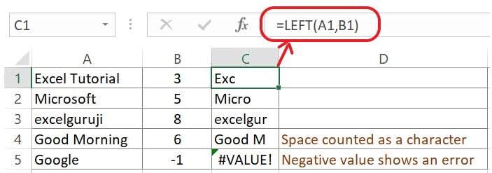
The LEFT function extracts a specified number of characters from the left side of a text string in a cell. In other words, it starts reading from the very first character on the left and returns however many characters you tell it to.

The basic syntax is:

=LEFT(text, [num_chars])

• text — the cell reference or text string you want to extract from
• num_chars — the number of characters to return (optional; defaults to 1 if omitted)

One key rule: the number of characters must always be greater than 0. If you omit it entirely, Excel automatically returns the first character.

You can apply it to a single cell:

=LEFT(A2)

Or across a range of cells:

=LEFT(A2:A4, 3)

How to Use the LEFT Function on a Single Cell

Let’s start with the most straightforward use case — extracting characters from one cell.

Step 1: Start the LEFT Function

1. Click on cell E2 (or any empty cell where you want the result to appear)
2. Type =LEFT
3. Double-click the LEFT command from the autocomplete dropdown

This opens the function and is ready for your input.

Step 2: Enter the Cell Reference and Press Enter

4. Click on cell A2 to select it as your input
5. Press Enter

The formula =LEFT(A2) uses the default behavior of the LEFT function and retrieves only the first character from cell A2. This is useful when, for example, you want to extract the first letter of a name or the first digit of a code.

How to Use the LEFT Function with a Defined Number of Characters

Most real-world scenarios require extracting more than just one character. Here’s how to specify exactly how many characters you want.

Step 1: Start the LEFT Function

1. Select cell E2
2. Type =LEFT
3. Double-click the LEFT command from the suggestion list

Note: The different parts of a LEFT formula are separated by a delimiter symbol — either a comma , or a semicolon ; — depending on your system’s Language/Regional Settings in Excel. If your formula throws an error, try switching between the two.

Step 2: Specify the Cell and Character Count

4. Type the cell reference followed by your delimiter and the number of characters: A2,3
5. Press Enter

The complete formula looks like this:

=LEFT(A2, 3)

This returns the first 3 characters from cell A2. For example, if A2 contains "Invoice-001", the result would be "Inv".

How to Use the LEFT Function on a Range of Cells

One of the most powerful features of the LEFT function is its ability to process multiple cells at once using a range reference. This is especially handy when you need to clean or standardize an entire column of data in one step.

Step 1: Start the LEFT Function

1. Select cell E2
2. Type =LEFT
3. Double-click the LEFT command

Step 2: Define the Range and Character Count

4. Enter the range reference and the number of characters with a delimiter: A2:A4,3
5. Press Enter

The complete formula:

=LEFT(A2:A4, 3)

This applies the LEFT function to every cell in the range A2 through A4, returning the first 3 characters from each one. If your column contains entries like "New York", "New Jersey", and "New Mexico", all three results would return "New" — a clean, consistent extraction in a single formula.

Practical Tips for Using the LEFT Function

Understanding the mechanics is one thing, but knowing when and how to apply it in real workflows is what makes this function truly useful:

• Combining with other functions: LEFT pairs naturally with functions like LEN, FIND, and IF. For example, =LEFT(A2, FIND("-", A2) - 1) extracts all characters before a hyphen — great for splitting product codes or order IDs.
• Case sensitivity: LEFT is not case-sensitive and does not modify the case of the extracted text. What’s in the cell is what you get.
• Numbers and dates: While LEFT works on numeric values, it treats them as text. Use it carefully with numbers or dates, as it may return unexpected results without first converting values to text using the TEXT function.
• Handling spaces: If your data has leading spaces, consider combining LEFT with TRIM to clean the text before extracting.

Conclusion

The Excel LEFT function is a straightforward but highly versatile tool for anyone who works with text data in spreadsheets. From extracting a single character to processing entire columns of strings, it handles a wide range of data-cleaning and formatting tasks with minimal effort. By mastering the LEFT function alongside its optional num_chars argument and range capabilities, you’ll significantly speed up your workflow when dealing with structured text data.

Ready to level up your Excel skills? Try combining LEFT with other text functions like RIGHT, MID, and LEN to unlock even more powerful text manipulation capabilities in your spreadsheets.