

Excel does not contain a built-in NOT CONTAINS function. To check if a cell does not contain text, use IF with NOT, ISNUMBER, and SEARCH: =IF(NOT(ISNUMBER(SEARCH("keyword",A1))),"True Value","False Value"). For counting or summing excluded text, use COUNTIF or SUMIFS with wildcard criteria.
Excel does not include a dedicated "does not contain" function, yet this is one of the most common conditions you need to apply when checking, counting, filtering, or summing worksheet data. The challenge lies in building equivalent logic using the tools available: the IF function combined with SEARCH or FIND, the COUNTIF function with wildcard patterns, SUMIFS for conditional totals, or filtering methods for visual data exploration. This article walks through each approach, explains when to use it, and shows you how to handle the complications that arise from partial matches, exact matches, and multiple excluded values.
Excel handles negation of text conditions through the not-equal-to operator (<>), which combines with wildcards to exclude cells containing specific text. When you need to check if a cell does not contain a particular substring, you have two main paths: formula-based logic that returns a result for each row, or filtering and counting functions that aggregate the data without adding a helper column. Understanding how each tool works and when partial text matching differs from exact matching will help you choose the right method for your spreadsheet task.
Creating a does-not-contain condition without a direct function
Excel provides no single function called "does not contain"; instead, you must combine the not-equal-to operator (<>) with other functions to express the negative condition. The reason is that most text-matching functions in Excel naturally check for presence (contains), so reversing that logic requires either a negation operator or a logical NOT statement. This design encourages you to think about your filtering or checking goal first, then select the tool that serves that goal—whether you need a label in each row, a count of excluded entries, a sum of amounts from excluded rows, or just a filtered view.
The most straightforward approach for checking whether a cell does not contain text is pairing the IF function with ISNUMBER and SEARCH. SEARCH scans a cell for a substring and returns the character position if found, or an error if not found. Wrapping SEARCH in ISNUMBER converts that result to TRUE (if the text was found) or FALSE (if not found). To reverse this and check for the absence of text, you wrap everything in NOT. The formula looks like this: IF(NOT(ISNUMBER(SEARCH("term", A1))), "action", "none"). This reads as: if the cell does not contain the term, return "action"; otherwise return "none".
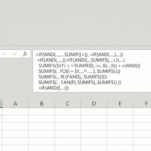
For counting cells that exclude certain text, COUNTIF is more direct. The formula COUNTIF(range, "<>term") counts all cells in the range that do not contain "term" as a substring anywhere in the cell. The asterisks act as wildcards, matching any number of characters before or after your search term. Without the wildcards—using just COUNTIF(range, "<>term")—the formula counts cells that do not contain "term" as an exact match, meaning a cell like "terminology" would be included in the count because it contains more than just "term".
Checking cells with IF, ISNUMBER, and SEARCH
When you need to evaluate each row and return a result (such as a label, a flag, or a number) based on whether the cell does not contain certain text, the IF function with ISNUMBER and SEARCH is the most common choice. This approach is flexible, works across all versions of Excel, and handles both text and partial matches naturally.
The formula structure is: =IF(NOT(ISNUMBER(SEARCH("keyword", A1))), "True Value", "False Value"). Here, SEARCH looks for "keyword" anywhere inside the cell A1. If found, SEARCH returns a number (the position of the first character of "keyword"). ISNUMBER wraps this and returns TRUE if a number is found (meaning the keyword was present) or FALSE if SEARCH returned an error (meaning the keyword was not found). NOT reverses the TRUE/FALSE result, so NOT(ISNUMBER(…)) returns TRUE when the keyword is NOT in the cell. Finally, IF branches on that TRUE/FALSE condition.
For example, suppose you have a list of order statuses in column B and you want to flag orders that do not contain the word "Completed" so you can review them. In cell C2, you would write: =IF(NOT(ISNUMBER(SEARCH("Completed", B2))), "Review", ""). If B2 contains "Order Completed on 2026-08-10", SEARCH finds "Completed", ISNUMBER returns TRUE, NOT reverses it to FALSE, and IF returns the empty string. If B2 contains "Order Pending", SEARCH does not find "Completed" and returns an error, ISNUMBER returns FALSE, NOT reverses it to TRUE, and IF returns "Review".
An alternative is to use IFERROR instead of NOT and ISNUMBER. The formula =IF(IFERROR(ISNUMBER(SEARCH("keyword", A1)), FALSE), "Found", "Not Found") is slightly wordier but achieves the same result by catching the SEARCH error and replacing it with FALSE. However, the NOT(ISNUMBER(…)) pattern is more widely taught and more compact.
One important detail: SEARCH is case-insensitive by default. So searching for "completed" will find "Completed", "COMPLETED", and "completed" all the same. If you need case-sensitive matching, replace SEARCH with FIND. The FIND function works identically except that FIND("Completed", A1) will only match the exact capitalization "Completed", not "completed" or "COMPLETED". Use FIND when your data requires strict case distinction.
Blank cells introduce a common gotcha. If A1 is empty, SEARCH("keyword", A1) returns an error, so ISNUMBER returns FALSE, NOT returns TRUE, and IF returns your "True Value"—meaning the formula correctly treats blank cells as "not containing" the keyword. However, if you want to exclude blank cells from your flagging (so that blank rows are not marked as needing review), add a second condition: =IF(AND(A1<>"", NOT(ISNUMBER(SEARCH("keyword", A1)))), "Review", ""). Now the formula only returns "Review" if the cell is non-blank AND does not contain the keyword.
Counting and summing cells that exclude specific text
When your goal is to report a total—how many cells do not contain a certain text, or what sum should be calculated from rows where a column does not contain a value—COUNTIF and SUMIFS are more efficient than IF formulas because they do the aggregation in a single cell without needing a helper column.
To count cells that do not contain text, use COUNTIF with the syntax =COUNTIF(range, "<>text"). The <> operator means "not equal to", and the asterisks are wildcards that match any characters. So COUNTIF(A:A, "<>cancelled") counts every cell in column A that does not contain the substring "cancelled" anywhere. If the range A2:A100 has 87 rows, and 5 of them contain the word "cancelled", the formula returns 82.
However, COUNTIF has a limitation: you cannot easily reference a cell to specify the text you want to exclude. If you want the exclusion term to come from a cell (like B1), you must concatenate: =COUNTIF(A:A, "<>"&B1&""). This works, but if you need to exclude multiple words, COUNTIF becomes cumbersome. For two exclusions, use COUNTIFS: =COUNTIFS(A2:A11, "<>word1", A2:A11, "<>word2"). This counts cells that do not contain "word1" AND do not contain "word2". Every cell must lack both words to be counted. If a cell contains either word, it is excluded from the count.
Wildcard behavior is critical to understand. The pattern "<>text" finds "text" anywhere in the cell (beginning, middle, or end). The pattern "<>text" (without wildcards) finds cells that are not exactly equal to "text" alone; a cell containing "text processing" or "pretext" would pass because the cell does not equal just "text". To match a whole word (like "cat" but not "catalog"), standard COUNTIF does not offer a built-in whole-word option, so you must either use the more complex SUMPRODUCT formula or apply filters.
For summing, SUMIFS allows multiple criteria across different ranges. If you have a revenue column (C) and a status column (B), and you want to sum revenue only from rows where status does not contain "cancelled", use: =SUMIFS(C:C, B:B, "<>cancelled"). The first range (C:C) is the sum range, and the second pair (B:B and the criteria) specify which rows to include. If status contains "Order Cancelled" or "Cancelled Shipment", those rows are excluded from the sum.

You can extend SUMIFS with multiple exclusion criteria. To sum revenue from rows where status does not contain "cancelled" AND does not contain "refunded", write: =SUMIFS(C:C, B:B, "<>cancelled", B:B, "<>refunded"). Both criteria must be true; if a row contains either word, it is not included in the sum.
Choosing the right Excel method for each task
Deciding whether to use IF, COUNTIF, SUMIFS, or filtering depends on what you want to achieve: flagging individual rows, reporting a count, calculating a total, or viewing a subset of data interactively.
Table: Excel does-not-contain methods
| Task goal | Recommended method | Best use case | Main limitation |
|---|---|---|---|
| Return a label or action when a cell does not contain specific text | IF with NOT and SEARCH or FIND | Conditional logic that branches based on text absence | Returns only one value per row; does not handle multiple exclusions as easily as filters |
| Count how many cells exclude a particular text string | COUNTIF with wildcard criteria | Reporting totals of non-matching entries without needing a helper column | Wildcard approach requires manual construction; COUNTIF does not directly read a cell reference as the exclusion criterion |
| Sum values based on cells that do not contain text | SUMIFS with exclusion criteria across multiple ranges | Totaling amounts from rows where a text column excludes certain words | SUMIFS adds complexity when combining multiple exclusion rules |
| View only rows where cells do not contain a value | AutoFilter or Advanced Filter with custom criteria | Temporarily hiding rows without creating formulas | Filters are interactive but temporary |
Use this table as a quick reference before you write any formula. If you are building a spreadsheet that will be maintained by others, prefer the method that requires the least explanation. A COUNTIF formula is self-contained and visible in a single cell. An IF formula forces anyone viewing the sheet to trace the logic across the range. AutoFilter is the most intuitive for users unfamiliar with formulas, but it requires manual interaction each time the data changes.
Matching rules that change does-not-contain results
The difference between partial text matching and exact text matching has a profound effect on how many rows your does-not-contain condition includes or excludes. Misunderstanding this difference is the most common reason formulas return unexpected counts or filter the wrong rows.
Consider a product list with entries: "Widget A", "Widget Pro", "Widget A Pro", and "Other". You want to count products that do not contain "Pro". Using COUNTIF(range, "<>Pro"), you count all cells that do not contain "Pro" anywhere. The result is 2: "Widget A" and "Other". The pattern "<>Pro" finds "Pro" anywhere in the text—at the start, middle, or end—so both "Widget Pro" and "Widget A Pro" are excluded.
If instead you use COUNTIF(range, "<>Pro"), you are asking for cells that are not exactly equal to "Pro". None of your cells contain only "Pro", so all 4 cells pass: "Widget A", "Widget Pro", "Widget A Pro", and "Other" are all included. The difference is dramatic: partial matching with wildcards narrows your result set, while exact matching with no wildcards broadens it.
This distinction matters for SUMIFS and COUNTIFS as well. If you sum revenue for items where product does not contain "cancelled", using "<>cancelled" excludes any item with "cancelled" anywhere. Without wildcards, using "<>Cancelled" includes all of these because none of them are exactly equal to the word "Cancelled" by itself.
Another subtlety is case sensitivity. COUNTIF and SEARCH are case-insensitive by default. COUNTIF(range, "<>pro") and COUNTIF(range, "<>Pro") produce identical results because Excel treats "pro", "Pro", "PRO" as the same. FIND is case-sensitive, so IF(NOT(ISNUMBER(FIND("Pro", A1))), …) will not match "pro" in lowercase. Use FIND when you must distinguish between "Pro" and "pro", or use EXACT with SEARCH for a case-sensitive contains check.
To prevent unexpected results, test your formula on a small subset (5–10 rows) and manually verify that the included and excluded rows match your intent. Pay special attention to cells containing partial matches of your exclusion term.
Handling multiple excluded words in one condition
Often a single exclusion term is not enough. You might need to exclude rows where the status does not contain "Completed" AND does not contain "Approved", or alternatively, exclude rows that contain any of several rejection reasons. The logic changes based on what you want.
When you want a row to be included only if it lacks ALL excluded terms, use AND logic. For IF formulas, write: =IF(AND(NOT(ISNUMBER(SEARCH("word1", A1))), NOT(ISNUMBER(SEARCH("word2", A1)))), "Include", "Exclude"). Both NOT-SEARCH conditions must be true. For COUNTIF, use COUNTIFS with both criteria.
When you want to exclude a row if it contains ANY of several terms, use OR logic. For IF: =IF(OR(ISNUMBER(SEARCH("word1", A1)), ISNUMBER(SEARCH("word2", A1))), "Exclude", "Include"). If either word is found, the cell is flagged for exclusion.
The decision rule is: AND logic is safer for COUNTIF because COUNTIFS directly supports it. OR logic is more difficult with COUNTIF but clearer with IF formulas. If you need OR logic with counting, use SUMPRODUCT or create a helper column with an IF formula, then count the helper column.
Filtering rows and fixing common formula errors
When you do not need formulas and simply want to see rows that do not contain certain text, filtering is often faster and more intuitive than building a formula. Excel offers two filtering methods: AutoFilter and Advanced Filter.
AutoFilter is the quick method. Select your data range, click Data > AutoFilter, and a dropdown arrow appears in each header cell. Click the dropdown in the column you want to filter, deselect any values containing your exclusion term, and click OK. The rows containing the excluded term are hidden. No formula is created; you are just controlling visibility.
Advanced Filter is more powerful but requires setting up a criteria range. Create a separate area of the sheet with a header row that matches a column name and a criteria row beneath it. To filter rows where Region does not contain "East", type the header "Region" in one cell and "<>East" in the cell below it. Then select your full data range, click Data > Advanced Filter, specify your data range and criteria range, and choose whether to filter in place or copy results to another location.
Common formula errors and their fixes:
COUNTIF returns too many rows. Check whether you used wildcards. COUNTIF(A:A, "<>text") counts cells not exactly equal to "text", which is almost everything. If you meant "does not contain text anywhere", use COUNTIF(A:A, "<>text") with wildcards.
SEARCH formula returns #VALUE! error. This happens when the search text is not found. Wrap SEARCH in IFERROR or use ISNUMBER(SEARCH(…)) to convert the error into FALSE.
IF formula flags the wrong rows. Verify that you are using NOT correctly. IF(NOT(…)) returns TRUE when the condition inside is FALSE.
SUMIFS sums more or fewer rows than expected. Double-check that every criteria range matches the corresponding criteria.
Blank cells are handled incorrectly. Blank cells may behave unexpectedly in COUNTIF. To exclude blanks explicitly, add a second criterion: COUNTIFS(A:A, "<>text", A:A, "<>"&"").
When Advanced Filter is better than formulas: if you need to filter rows interactively and save the hidden rows for later analysis, Advanced Filter is faster. If you need a permanent calculated result, formulas are better because they update automatically when data changes.
Test your formula on a small sample first. Copy the formula down a few rows, manually verify that each result is correct, and only then apply it to the full range. This habit catches logic errors early and prevents incorrect results from spreading across hundreds of rows.
When you need to verify an unexpected formula result, add a helper column with =SEARCH("term", A1) and examine the raw output. If SEARCH returns a number, the term was found; if it returns #VALUE!, the term was not found. This diagnostic step clarifies what SEARCH is actually seeing.
Build and test your first does-not-contain formula on a small sample of 5 to 10 rows, checking each result manually against the data before scaling it to your full dataset. This prevents mistakes that are expensive to fix on large worksheets and builds confidence that the formula logic is correct for your specific data patterns.
FAQ
Can Excel does not contain formulas work with numbers?
Yes. Excel does-not-contain logic can be applied when cells contain numbers by using the same conditional methods, although these formulas are most commonly used for text checks. IF, COUNTIF, and SUMIFS can evaluate conditions involving cell values depending on the formula structure and criteria you use.
Does Excel text exclusion work with multiple worksheets?
Yes. Excel text exclusion logic can be used with data across multiple worksheets when formulas reference the correct cells or ranges. The same IF, COUNTIF, and SUMIFS approaches apply, but each formula must point to the worksheet ranges containing the data you want to evaluate.
Can Excel check for missing text without using formulas?
Yes. Excel can check for missing text without formulas by using filtering methods such as AutoFilter or Advanced Filter. These tools let you hide rows containing specific values and view the remaining data without adding helper columns or calculated results.
Why does an Excel does-not-contain formula return the wrong result?
A does-not-contain formula often returns unexpected results because of matching rules. Check whether you need partial matching with wildcards like "<>text" or exact matching with "<>text". Also verify NOT logic, blank cell handling, and whether the formula uses the correct ranges and criteria.