

The Quick Analysis tool in Excel appears after you select a compatible range of cells. Look for the small lightning-bolt icon near the lower-right corner of the selected data range, then click it to open Quick Analysis options. You can also press Ctrl + Q after selecting data.
If you selected a group of cells in Microsoft Excel and cannot find the Quick Analysis button, the problem is usually that you are looking in the wrong place. Quick Analysis is not a Ribbon command; it appears as a small floating icon near the bottom-right corner of a selected data range. This guide shows how to open Quick Analysis, use its main options, and restore it when the icon or shortcut does not appear.
The Quick Analysis tool in Excel appears after you select a compatible range of cells. Look for the small lightning-bolt icon at the lower-right edge of the selection, then click it to open the Quick Analysis gallery with options for Formatting, Charts, Totals, Tables/PivotTables, and Sparklines.
Finding the Quick Analysis button in Excel
Many beginners search through Excel tabs because they expect Quick Analysis to be another command in the Ribbon. It works differently: the feature is context-sensitive, meaning Excel displays it only when you select data that can be analyzed.
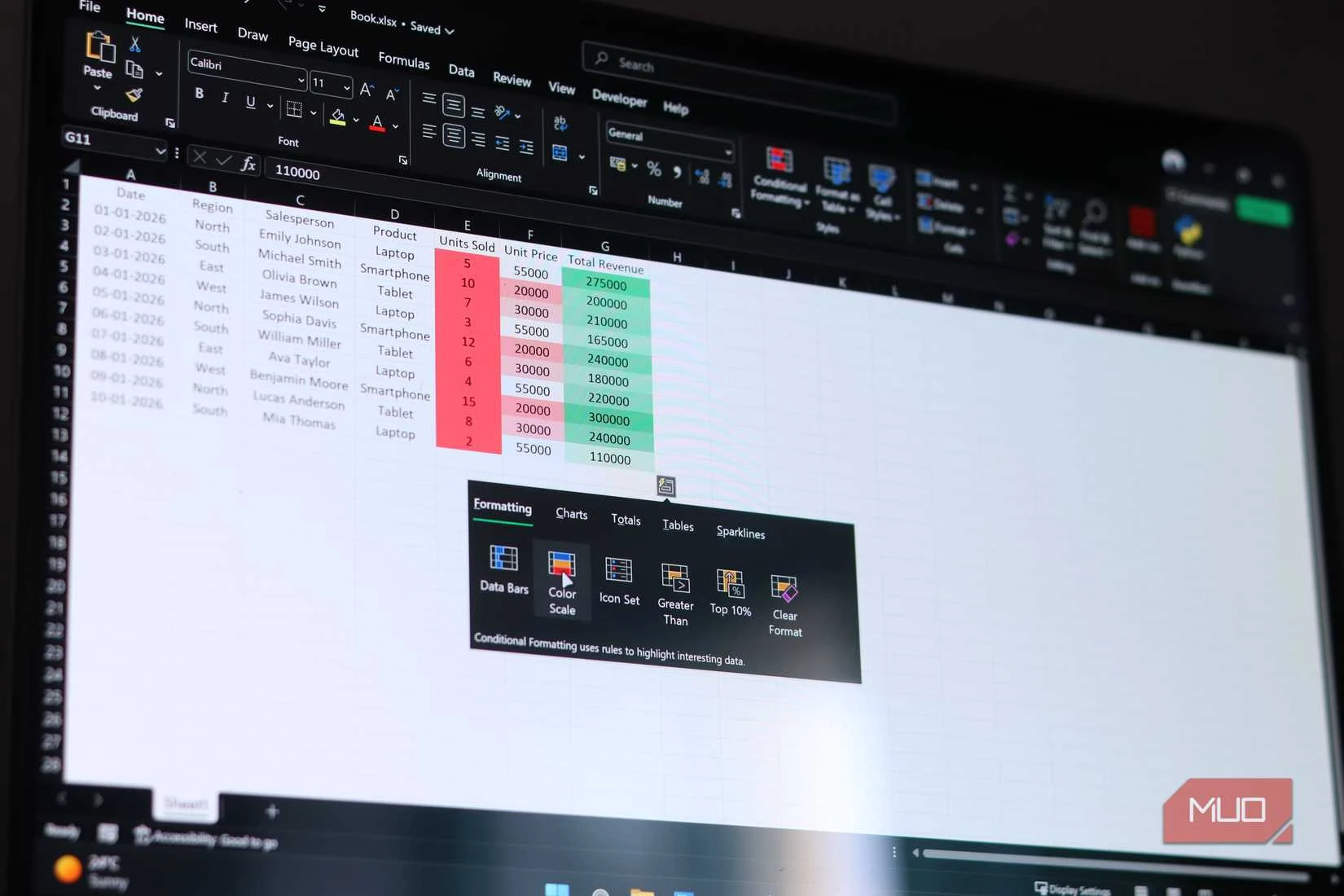
The icon normally appears beside the highlighted cells, close to the lower-right corner of the selected range. It is a small button that opens the Quick Analysis gallery when clicked.
The fastest way to check is to select your data first, then look at the edge of the selection rather than searching menus.
A suitable selection usually contains actual data values, such as a list of sales amounts, dates, categories, or other organized worksheet information. A blank area, a single empty cell, or a selection that does not contain useful data may not trigger the icon.
Opening Quick Analysis from a worksheet
Once the correct data range is selected, opening Quick Analysis takes only a few seconds. The feature is designed for quick decisions while viewing worksheet data.
To open it with a mouse:
- Select the cells you want to analyze.
- Find the small Quick Analysis button near the bottom-right corner of the highlighted area.
- Click the button to open the gallery.
- Choose a category such as Formatting, Charts, Totals, Tables, or Sparklines.
- Select a preview option to apply the result.
You can also use the keyboard shortcut after selecting your data. Press Ctrl + Q to open Quick Analysis. The shortcut works after a compatible selection is active; it is not a general Excel search command.
Fixing a missing Quick Analysis button
When Quick Analysis is missing, changing random Excel menus usually wastes time. Check the selection, feature setting, and Excel version in that order.
For Mac users, the main check is also the selection-based behavior. Quick Analysis is not a Ribbon button that you browse to. Select a suitable data range and look around the selected cells for the floating option. If you use Excel on macOS, the related workflow is covered in this Mac Excel Quick Analysis Tool guide.
Select a real data range in Excel today and open Quick Analysis with the lightning-bolt icon or Ctrl + Q; this immediately confirms whether the feature is available and lets you choose the right analysis option for your current worksheet task.