Understanding Supply and Demand Curves with Excel

This guide delves into the practical application of supply and demand principles, specifically demonstrating how to visualize and analyze these economic concepts using Microsoft Excel. We will explore how to graph supply and demand curves, interpret their movements, and understand the underlying economic forces, particularly focusing on the concept of elasticity and the impact of exogenous shocks. This analysis is crucial for anyone seeking to grasp market dynamics, whether they are students of economics or professionals working with economic data.

Part 7.1: Graphing Supply and Demand Diagrams in Excel

Before we can effectively plot supply and demand curves, it’s essential to convert data, often presented in natural logarithms for economic analysis, back into their original numerical values. This process allows for a more intuitive understanding of price and quantity relationships.

To begin, we’ll create two new variables representing the actual prices (P) and quantities (Q). Subsequently, we will generate separate line charts for P and Q, with time (in years) on the horizontal axis, ensuring clear labeling of the vertical axes. This visualization will mirror Figure 1 in the referenced paper.

Let’s consider a simplified model for watermelon supply and demand, where Q represents quantity in millions and P denotes the price per thousand watermelons. The supply curve is defined by the equation:
log P = -2.0 + 1.7 log Q (Supply curve)

And the demand curve is described by:
log P = 8.5 - 0.82 log Q (Demand curve)

To plot these curves, we need to generate a series of points. We’ll start with the variables in their natural log format and then convert them to actual prices and quantities.

1. Data Preparation:

   • In a new spreadsheet tab, create a table with columns for Q, Log Q, Supply (log P), Demand (log P), Supply (P), and Demand (P).
   • Populate the Q column with values ranging from 20 to 100, in increments of 5 (representing 20 million to 100 million watermelons).
   • Convert Q values to their natural log format in the Log Q column.
   • Using the provided supply and demand equations and the Log Q values, calculate the corresponding log P values for both supply and demand.
   • Employ Excel’s EXP function to convert these log P values into actual prices (P) for the ‘Supply (P)’ and ‘Demand (P)’ columns.

2. Plotting the Curves:

   • Create a line chart with price (P) on the vertical axis and quantity (Q) on the horizontal axis.
   • Add both the calculated supply and demand curves to the chart, ensuring they are clearly labeled using a legend.

Impact of Exogenous Shocks: The Case of a Negative Supply Shock

An exogenous event is one that originates from outside a system and influences it, rather than being a result of the system’s internal workings. During the period of 1930–1951, the watermelon market experienced a negative supply shock due to the Second World War, which diverted production inputs. This external event shifted the entire supply curve.

Before proceeding, consider sketching a supply and demand diagram to illustrate the expected impact of such a shock on price and quantity, assuming all other factors remain constant. For a real-world example, consider how oil shocks in the 1970s shifted the supply curve in the oil market, as discussed in Section 7.13 of Economy, Society, and Public Policy.

Now, let’s quantify the effect of this negative supply shock using our Excel model. Assume the supply curve after the shock is represented by:
log P = -2.0 + 1.7 log Q + 0.4

1. Updating the Supply Curve:

   • Add a new column to your table for ‘New supply (log P)’ and another for ‘New supply (P)’, reflecting the updated supply equation.
   • Incorporate the ‘New supply (P)’ data into your existing line chart, labeling this new curve clearly. Verify that the chart visually represents the expected shift.

2. Analyzing Surplus Changes:

   • Based on your chart, analyze the changes in total surplus, consumer surplus, and producer surplus resulting from this supply shock. The old equilibrium was approximately Q = 64.5, P = 161.3, and the new equilibrium is Q = 55.0, P = 183.7. Consumer and producer surplus concepts are further elaborated in Sections 7.6 and 7.11 of Economy, Society, and Public Policy.

Part 7.2: Interpreting Supply and Demand Curves

Expressing economic relationships in natural log form is advantageous because the coefficients directly represent elasticities. In an equation like log Y = a + b log X, the coefficient b signifies the elasticity of Y with respect to X, indicating the percentage change in Y for a 1 percent change in X. The concept of elasticity is further explored in Section 7.8 of The Economy.

Recall the supply and demand equations from Part 7.1:

• Supply curve: log P = -2.0 + 1.7 log Q
• Demand curve: log P = 8.5 - 0.82 log Q

1. Calculating Elasticities:
   • Price Elasticity of Supply: Rearrange the supply equation to express log Q in terms of log P. Then, calculate the price elasticity of supply (the percentage change in quantity supplied divided by the percentage change in price) and comment on its magnitude.
   • Price Elasticity of Demand: Calculate the price elasticity of demand similarly and discuss its size in absolute value.

Economic Interpretation of Supply and Demand Equations

Let’s examine the estimated supply equation for watermelons from the paper:
log Q_t = 2.42 + 0.58 log P_{t-1} - 0.32 log C_{t-1} - 0.12 log T_{t-1} + 0.07 CP_t - 0.36 WW2_t

Here, Q_t is the quantity of watermelons supplied in the current period, P_{t-1} is the price of watermelons in the previous period, C_{t-1} is the price of cotton in the previous period, T_{t-1} is the price of vegetables in the previous period, CP is a dummy variable (1 if the government cotton-acreage-allotment program was active, 0 otherwise), and WW2 is a dummy variable (1 if the US was involved in WWII, 0 otherwise).

Information regarding government farm programs for cotton during this era can be found in the report ‘The cotton industry in the United States’.

The variables C, T, CP, and WW2 are exogenous factors influencing farmers’ decisions, thereby affecting the endogenous variables P and Q. As depicted in Figure 7.3, changes in endogenous variables lead to movements along the supply curve (right-hand panel), while exogenous shocks shift the entire curve by altering its intercept (left-hand panel).

Supply curve: Dummy variables shift the entire curve (left-hand panel), while changes in endogenous variables move along the curve (right-hand panel).

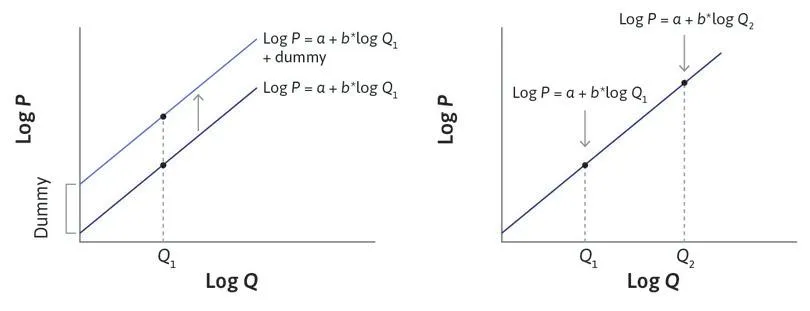
Figure 7.3: Supply curve analysis showing shifts versus movements.

1. Interpreting Supply Equation Coefficients: Referencing Figure 7.4, provide an economic interpretation for each variable’s coefficient in the supply equation. Explain its effect on farmers’ supply decisions and, where applicable, relate it to an elasticity.

   Variable	Coefficient	95% Confidence Interval
   P (watermelon price)	0.580	[0.572, 0.586]
   C (cotton price)	–0.321	[–0.328, –0.314]
   T (vegetable price)	–0.124	[–0.126, –0.122]
   CP (cotton program)	0.073	[0.068, 0.077]
   WW2 (WWII)	–0.360	[–0.365, –0.355]

   Figure 7.4: Supply equation coefficients and their confidence intervals.

Now, let’s analyze the demand curve (equation (3) in the paper), which specifies per capita demand in terms of price and other variables. The intercept is denoted by α₀.
log (X_t/N_t) = α₀ - 1.13 log(P_t) + 1.75 log(Y_t/N_t) - 0.97 log F_t

1. Interpreting Demand Equation Coefficients: Using the demand equation and Figure 7.5, provide an economic interpretation for each coefficient, relating it to elasticity where appropriate.

   Variable	Coefficient	95% Confidence Interval
   P (watermelon price)	–1.125	[–1.738, –0.512]
   Y/N (per capita income)	1.750	[0.778, 2.722]
   F (railway freight costs)	–0.968	[–1.674, –0.262]

   Figure 7.5: Demand equation coefficients and their confidence intervals.

Addressing Simultaneity in Economic Models

The simultaneity problem arises when variables in a model affect each other reciprocally. In supply and demand models, price influences quantity supplied and demanded, and simultaneously, quantity affects price. This makes it challenging to estimate supply and demand curves using only price and quantity data, as the independent variables are not truly independent. Figure 7.6 illustrates how various supply and demand curve shifts can explain the same observed data points.

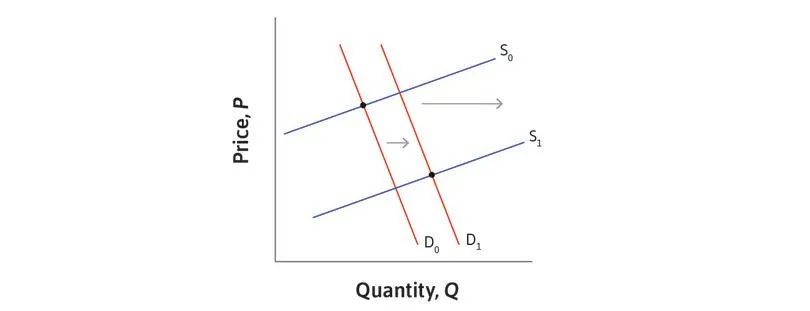
Many possible supply and demand curves can explain the data. Many possible supply and demand curves can explain the data.Many possible supply and demand curves can explain the data.

Figure 7.6: Demonstrating how multiple supply and demand curves can fit the same data.

To overcome this, we seek an exogenous variable that impacts one equation but not the other, allowing us to isolate shifts. The Second World War served as an exogenous supply shock in Part 7.1, influencing watermelon production but not demand. Figure 7.7 demonstrates how such supply shocks can help identify the demand curve. By assuming a linear demand curve, we can infer its shape from the points revealed by the supply shock. Similarly, exogenous demand shocks aid in identifying the supply curve.

Using exogenous supply shocks to identify the demand curve.

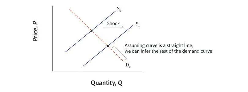
Figure 7.7: Identifying the demand curve using exogenous supply shocks.

1. Examples of Exogenous Demand Shocks: Considering the watermelon market model, provide two examples of exogenous demand shocks and explain why they qualify as exogenous.