Mastering Excel Slicers: A Complete Guide for Efficient Data Filtering

Slicers in Excel provide a visual and interactive way to filter data in tables and PivotTables. Beyond simple filtering, slicers allow you to quickly see which filters are currently applied, making it easier to understand and manage the data displayed.

Introduction to Slicers

Slicers are user-friendly filter controls that let you select data categories with a single click. They are especially useful for PivotTables, as they visually indicate which data is currently being filtered. This guide will walk you through creating, formatting, and managing slicers to optimize your Excel workflow.

Creating a Slicer

Follow these steps to insert a slicer for a table or PivotTable:

1. Click anywhere within your table or PivotTable.
2. Go to the Insert tab and select Slicer.
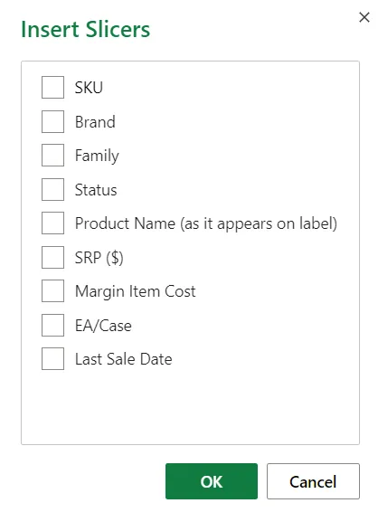
3. In the Insert Slicer dialog box, check the boxes for the fields you want to display and click OK.
4. A slicer will appear for each selected field. Clicking any slicer button automatically applies that filter to the connected table or PivotTable.

Tips:

• To select multiple items, hold Ctrl (Windows) or Command (Mac) while selecting.
• To clear the slicer filter, click the Clear Filter button within the slicer.

Formatting and Customizing Slicers

You can adjust slicer options using the Slicer tab (Excel 2013 and later) or the Design tab (Excel 2016 and earlier) on the ribbon.

• Choose a color style that suits your worksheet design.
• Resize a slicer by selecting and dragging its corner handles.
• If you already have a slicer on a PivotTable, you can reuse it to filter another PivotTable that shares the same data source.

Connecting a Slicer to Multiple PivotTables

To share a slicer across different PivotTables:

1. Ensure the new PivotTable uses the same data source as the existing one.
2. Select the slicer you want to share. The Slicer tab will appear.
3. Click Report Connections (or PivotTable Connections), then check the PivotTables you want to link.
4. Click OK to apply.

Disconnecting or Removing a Slicer

To disconnect a slicer from a PivotTable:

1. Click anywhere in the PivotTable. The PivotTable Analyze tab will appear.
2. Select Filter Connections, then uncheck the PivotTables you want to disconnect.
3. Confirm with OK.

To remove a slicer entirely:

• Select the slicer and press Delete, or
• Right-click the slicer and choose Remove.

Understanding Slicer Components

A slicer typically includes the following elements:

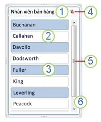PivotTable slicer components showing filter buttons, title, scroll bar, and resize handles	Description
1. Slicer title	Indicates the category of items in the slicer
2. Unselected filter button	Represents an item not included in the filter
3. Selected filter button	Represents an item included in the filter
4. Clear Filter button	Removes all filters by selecting all items
5. Scroll bar	Allows scrolling when there are more items than visible
6. Resize/move handles	Adjust the slicer’s size and position

Using Slicers in Excel for Web

Only local PivotTable slicers are available in Excel for Web. To create slicers for tables, PivotTable data models, or Power BI PivotTables, use Excel for Windows or Excel for Mac.

1. Click anywhere in the PivotTable.
2. Go to the PivotTable Analyze tab and select Slicer.
3. Choose the fields you want in the Insert Slicer dialog and click OK.

Tips:

• Hold Ctrl to select multiple items in the slicer.
• Click Clear Filter to remove applied filters.

Conclusion

Slicers are an essential tool for efficient data analysis in Excel, providing both visual clarity and quick filtering capabilities. By learning to insert, format, connect, and manage slicers, you can significantly improve your productivity and data insights. Start integrating slicers into your workflow today to take control of your PivotTables and tables like a pro.

References

• Microsoft Excel Slicer Overview
• Filter Data in PivotTables
• Excel Tech Community