Excel’s ability to process and visualize data is unparalleled, making it an indispensable tool for professionals across industries. While basic functions are widely known, mastering advanced techniques can significantly boost efficiency and analytical depth. One such powerful technique is calculating a rolling average, a method that smooths out data fluctuations and reveals underlying trends. This guide will walk you through how to calculate rolling averages in Excel, enabling you to work smarter, not harder.
A rolling average, also known as a moving average, is a series of averages of different subsets of a full data set. It’s particularly useful when analyzing data that exhibits cyclicality or seasonality, such as daily sales or monthly performance metrics. By averaging data over a specified period and continuously updating this average as new data points become available, rolling averages help to smooth out short-term fluctuations and highlight longer-term trends. This makes it easier to discern genuine upward or downward movements from temporary variations. For instance, a restaurant owner can use a rolling average of daily customers to see if business is truly growing, even with the natural weekly fluctuations of more customers on weekends. Similarly, a retail manager can track monthly sales trends more accurately by using a rolling average that accounts for holiday sales spikes.
Calculating Rolling Averages Manually in Excel
The manual method for calculating a rolling average in Excel is straightforward and offers granular control. It involves creating a new column for your rolling averages and using the AVERAGE function in conjunction with Excel’s powerful cell referencing capabilities.
Let’s consider an example using daily sales figures. Suppose you have daily sales data for “SnackWorld” cookies, which shows considerable variation day by day, often peaking mid-week. To get a clearer picture of the overall sales trend, you can implement a 7-day rolling average.
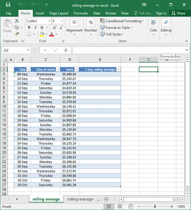
To calculate the 7-day rolling average, you would create a new column. In the first cell where a full seven days of data are available (e.g., cell E9, corresponding to September 15th), you would enter a formula like this: