When you’re working with large datasets in Excel, messy text is one of the most common headaches you’ll encounter. Maybe you have a column of names and job titles separated by a comma, or email addresses you need to parse, or URLs where you only need a specific segment. Whatever the case, knowing how to remove text before or after a specific character in Excel is a core data-cleaning skill that can save you significant time.
Excel gives you several ways to tackle this — from the quick-and-dirty Find & Replace method to the precision of nested formulas. This guide walks through all of them, so you can pick the right tool for your situation.
3 Methods to Remove Text Before or After a Specific Character
Before diving into advanced formulas, it helps to understand what we’re working with. Suppose you have a column where each cell contains a name and an age separated by a comma — for example, John, 28. You want to strip out everything after the comma and keep only the name.
Here are three reliable methods to accomplish this in Excel.
Method 1: Find & Replace with Wildcard Characters
The Find & Replace tool is the fastest option when you want to modify data directly in your cells without writing a formula. It leverages Excel’s wildcard character *, which matches any sequence of characters.
Step 1: Select your data range. Highlight the cells you want to modify, then navigate to the Home tab on the ribbon.
Step 2: Open Find & Replace. Click Find & Select in the Editing group, then choose Replace from the dropdown. Alternatively, press Ctrl + H to open the dialog box directly.
Step 3: Enter your search criteria. In the Find what field, use one of these wildcard patterns depending on what you want to remove:
- *`,` — removes everything before** a comma (including the comma itself)
- *`,` — removes everything after** a comma (including the comma itself)
- *`AC` — removes text between** two specific characters
Leave the Replace with field completely blank, then click Replace All.
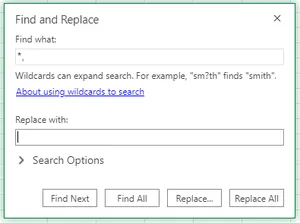
A confirmation dialog will tell you how many replacements were made. Check your cells to verify the results look correct.
Note: Find & Replace modifies your data in place. Always work on a copy of your data or make sure you can undo with Ctrl + Z if something goes wrong.
Method 2: Flash Fill — Pattern-Based Auto-Complete
Flash Fill is one of Excel’s most underrated features. Once it detects a pattern in what you’re typing, it automatically fills in the remaining cells. No formulas required.
Step 1: Type the expected result manually. In the cell adjacent to your first data entry — say, column B if your data is in column A — type the result you want. For example, if cell A1 contains John, Manager and you only want Manager, type Manager in B1.

Step 2: Let Excel detect the pattern. Move to B2 and start typing the expected result for the second row. Excel will analyze the pattern between your original data and what you’ve typed. If it recognizes a consistent rule, it will display a gray preview of suggested values for all remaining rows.
Step 3: Accept the suggestions. Press Enter to apply Flash Fill across all rows. If Excel doesn’t suggest anything automatically, you can trigger it manually via Data > Flash Fill or by pressing Ctrl + E.
Flash Fill works best when your data is consistent. If your delimiter or structure varies across rows, you may get unpredictable results — in that case, use a formula instead.
Method 3: Using Excel Formulas (SUBSTITUTE, LEFT, RIGHT)
Formulas give you the most control and flexibility. Unlike Find & Replace, they’re non-destructive — your original data stays untouched, and the cleaned result appears in a separate column.
Using the SUBSTITUTE Function
SUBSTITUTE replaces a specific piece of text within a string with something else. To “remove” text, you simply replace it with an empty string "".
Syntax:
=SUBSTITUTE(cell_reference, "text_to_remove", "")For example, if A2 contains Hello, World and you want to remove the word Hello, enter this in B2:
=SUBSTITUTE(A2, "Hello", "")Press Enter, and B2 will display , World. You can then apply TRIM to clean up leading spaces if needed.
How to Delete Everything After a Specific Character
When you need to extract only the text that appears before a delimiter, combine the LEFT and SEARCH functions.
The formula:
=LEFT(cell, SEARCH("character", cell) - 1)How it works:
SEARCH(",", A2)finds the position of the comma in the text- Subtracting
1ensures the comma itself is excluded LEFT(A2, ...)extracts that many characters from the start of the string
Example: If A2 contains Smith, 34, entering =LEFT(A2, SEARCH(",", A2) - 1) in B2 returns Smith.
Handling missing characters: If a cell doesn’t contain the delimiter, SEARCH will return a #VALUE! error. Wrap the formula in IFERROR to handle this gracefully:
=IFERROR(LEFT(A2, SEARCH(",", A2) - 1), A2)This returns the original text unchanged when no delimiter is found. You can also swap "," for any other character — "@" for email domains, "/" for URL segments, " " for spaces, and so on.
How to Delete Everything Before a Specific Character
To keep only the text that comes after a delimiter, use the RIGHT, LEN, and SEARCH functions together.
The formula:
=RIGHT(cell, LEN(cell) - SEARCH("character", cell))How it works:
SEARCH(",", A2)locates the position of the delimiterLEN(A2)returns the total length of the string- Subtracting the position from the length gives the number of characters after the delimiter
RIGHT(A2, ...)extracts exactly that many characters from the end
Example: If A2 contains Smith, 34, the formula returns 34 (note the leading space). To remove that space, wrap the whole thing in TRIM:
=TRIM(RIGHT(A2, LEN(A2) - SEARCH(",", A2)))Case sensitivity: By default, SEARCH is case-insensitive. If you need to match a specific case, replace it with FIND:
=TRIM(RIGHT(A2, LEN(A2) - FIND(",", A2)))Removing Text After the Nth Occurrence of a Character
When your text contains multiple instances of the same delimiter — for example, New York, USA, 2024 — you might want to remove everything after the second comma, not the first. This requires a slightly more advanced formula.
The formula:
=LEFT(cell, FIND("#", SUBSTITUTE(cell, "char", "#", n)) - 1)How it works:
SUBSTITUTE(A2, ",", "#", 2)replaces only the 2nd occurrence of the comma with a unique placeholder character#FIND("#", ...)locates the position of that placeholderLEFT(A2, ... - 1)extracts everything to the left of it
Example: If A2 contains John, New York, Manager, entering =LEFT(A2, FIND("#", SUBSTITUTE(A2, ",", "#", 2)) - 1) returns John, New York.
Replace 2 with whichever occurrence number you need to target.
Removing Text Before the Nth Occurrence of a Character
Conversely, to keep only what comes after the nth delimiter, combine RIGHT, SUBSTITUTE, and FIND:
=RIGHT(SUBSTITUTE(A2, ",", "#", 2), LEN(A2) - FIND("#", SUBSTITUTE(A2, ",", "#", 2)))Again, wrap in TRIM to clean up any leading spaces:
=TRIM(RIGHT(SUBSTITUTE(A2, ",", "#", 2), LEN(A2) - FIND("#", SUBSTITUTE(A2, ",", "#", 2))))Drag the formula down your column to apply it to all rows in your dataset.
Troubleshooting Common Errors
Even with the right formula, you might run into a few issues. Here’s how to handle the most common ones:
#VALUE! errors from SEARCH or FIND: This happens when the character you’re searching for doesn’t exist in the cell. Use IFERROR to return a fallback value — typically the original text — instead of displaying an error.
Unexpected results or wrong outputs: Double-check whether you should be using SEARCH (case-insensitive, supports wildcards) or FIND (case-sensitive, no wildcards). A mismatch here is a frequent source of confusion. Also confirm your cell references are correct and that there are no hidden spaces in your data — apply TRIM as a pre-processing step if needed.
Flash Fill producing inconsistent results: If your source data isn’t structured uniformly, Flash Fill may misread the pattern. In that case, fall back to a formula-based approach for greater reliability.
Conclusion
Whether you’re cleaning up imported data, parsing delimited strings, or extracting just the information you need, Excel gives you multiple paths forward. Find & Replace is ideal for quick, one-time edits directly on your data. Flash Fill works great when your data is consistent and you want a no-formula solution. And formulas using LEFT, RIGHT, SEARCH, FIND, and SUBSTITUTE offer the most precision and flexibility — especially when you need to handle edge cases or target specific occurrences of a delimiter.
Start with the method that fits your dataset and comfort level, and don’t hesitate to combine techniques — for example, using TRIM around a RIGHT formula to ensure clean output. Once you’ve mastered these tools, you’ll be able to clean data in Excel faster and with far greater confidence.