Working with extensive text data in spreadsheets often requires isolating specific segments for analysis. Microsoft Excel and Google Sheets offer various effective methods to extract text situated between two characters or words. This guide provides a comprehensive overview of the most efficient techniques to achieve this.
Extracting Text Between Two Distinct Characters in Excel
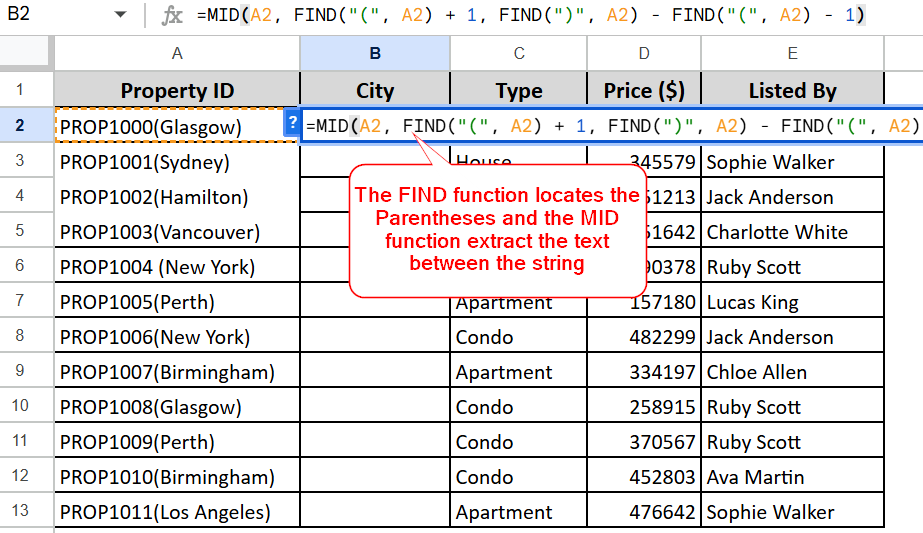
A versatile formula can be employed to extract text bounded by two different characters. The general structure is as follows:
=MID(cell, SEARCH(char1, cell) + 1, SEARCH(char2, cell) - SEARCH(char1, cell) - 1)
For instance, to retrieve text enclosed in parentheses from cell A2, the formula would be:
=MID(A2, SEARCH("(", A2)+1, SEARCH(")", A2) - SEARCH("(", A2) -1)
This method is adaptable for extracting text between various delimiters like braces {}, square brackets [], or angle brackets <>.
Tip: If your extracted data consists of numbers and you need them to be treated as numerical values rather than text strings, you can apply a simple arithmetic operation, such as multiplying by 1 or adding 0, to the formula’s result.
=MID(A2, SEARCH("(", A2)+1, SEARCH(")", A2) - SEARCH("(", A2) -1) *1
This ensures correct numerical formatting and alignment within your spreadsheet.
Understanding the Formula Mechanics
The core of this extraction process lies in Excel’s MID function, which extracts a specified number of characters from a text string, starting at a defined position. The MID function syntax is:
MID(text, start_num, num_chars)
- text: This refers to the cell containing the original string (e.g., A2).
- start_num: This is calculated by finding the position of the opening character using the
SEARCHfunction and adding 1 to it. This positions the extraction point immediately after the opening delimiter:SEARCH("(", A2) + 1. - num_chars: This determines how many characters to extract. It’s calculated by finding the position of the closing character and subtracting the position of the opening character. An additional subtraction of 1 excludes the closing delimiter itself:
SEARCH(")", A2) - SEARCH("(", A2) - 1.
By combining these elements, the MID function precisely extracts the desired text segment. Since MID inherently returns a text string, converting numerical results to actual numbers is necessary if required.
Extracting Text Between Two Strings or Words in Excel
Similar to extracting between characters, extracting text between specific words or strings involves a slightly modified formula. The key adjustment is incorporating the length of the delimiter words using the LEN function to ensure these words are excluded from the final extracted text.
=MID(cell, SEARCH(word1, cell) + LEN(word1), SEARCH(word2, cell) - SEARCH(word1, cell) - LEN(word1))
For example, to extract text situated between the words “start” and “end” from cell A2, the formula would be:
=IFERROR(MID(A2, SEARCH("start ", A2) + LEN("start "), SEARCH(" end", A2) - SEARCH("start ", A2) - LEN("start ")), "")
This formula utilizes IFERROR to gracefully handle cases where the specified delimiter words are not found in the text.
Extracting Text Between Identical Characters in Excel
When you need to extract text between two instances of the same character, such as double quotes, a nested SEARCH function is employed. The general formula is:
MID(cell, SEARCH(char, cell) + 1, SEARCH(char, cell, SEARCH(char, cell) + 1) - SEARCH(char, cell) - 1)
For instance, to extract text between double quotes (") in cell A2, you would use:
=MID(A2, SEARCH("""", A2) + 1, SEARCH("""", A2, SEARCH("""",A2) + 1) - SEARCH("""", A2) - 1)
Note on Double Quotes: In Excel formulas, a literal double quote is represented by entering two double quotes together ("") within the formula. Alternatively, you can use the CHAR function with its corresponding ASCII code (34 for a double quote):
=MID(A2, SEARCH(CHAR(34), A2) + 1, SEARCH(CHAR(34), A2, SEARCH(CHAR(34),A2) + 1) - SEARCH(CHAR(34), A2) - 1)
Deconstructing the Formula for Identical Characters
The MID function arguments are applied as follows:
- text: The source cell (A2).
- start_num: Calculated as the position of the first occurrence of the character plus one:
SEARCH(""""", A2) + 1. - num_chars: This is the more complex part, involving a nested
SEARCH. The innerSEARCHfinds the position of the second occurrence of the character. The outerSEARCHuses this position to determine the starting point for the count. The final calculation subtracts the position of the first character from the second and then subtracts 1 to exclude the second character itself:SEARCH(""""", A2, SEARCH(""""",A2) + 1) - SEARCH(""""", A2) - 1.
This structure allows MID to extract the exact text segment between the two specified characters.
Case-Sensitive Text Extraction in Excel
Excel offers both case-insensitive (SEARCH) and case-sensitive (FIND) functions for locating text. When the delimiter’s case is critical, FIND is the appropriate choice.
Consider extracting text between two uppercase “X” characters. Using SEARCH might yield incorrect results if a lowercase “x” is present:
=MID(A2, SEARCH("X", A2) +1, SEARCH("X", A2, SEARCH("X",A2) +1) - SEARCH("X", A2) -1) +0
In contrast, the FIND function ensures case sensitivity:
=MID(A2, FIND("X", A2) +1, FIND("X", A2, FIND("X",A2) +1) - FIND("X", A2) -1) +0
This FIND-based formula correctly isolates text specifically between uppercase “X” characters.
Simplified Extraction in Excel 365 with TEXTBEFORE and TEXTAFTER
Excel 365 introduces the TEXTBEFORE and TEXTAFTER functions, significantly simplifying text extraction. To extract text between two characters, these functions can be used in conjunction:
=TEXTBEFORE(TEXTAFTER(cell, char1), char2)
For example, extracting text between parentheses is remarkably straightforward:
=TEXTBEFORE(TEXTAFTER(A2, "("), ")")
Similarly, extracting text between double quotes becomes:
=TEXTBEFORE(TEXTAFTER(A2, """"), """")
Both TEXTAFTER and TEXTBEFORE are case-sensitive by default. To perform a case-insensitive extraction, you can utilize the match_mode argument, setting it to 1 or TRUE.
=TEXTBEFORE(TEXTAFTER(A2, "x ", ,1), " x", ,1) +0
This case-insensitive formula will recognize both “x ” and ” x” as delimiters.
How TEXTBEFORE and TEXTAFTER Work Together
The process involves working from the inside out. The TEXTAFTER function first extracts all text following the initial delimiter. The resulting substring is then passed to the TEXTBEFORE function, which isolates the text preceding the second delimiter within that substring.
Extracting Text Between Characters in Google Sheets
Google Sheets fully supports the MID and SEARCH function combinations that are effective in Excel. Therefore, you can use the same formulas for text extraction.
For instance, to extract text between square brackets [] in cell A2:
=MID(A2, SEARCH("[", A2)+1, SEARCH("]", A2) - SEARCH("[", A2) -1)
And to extract text between two commas:
=MID(A2, SEARCH(",", A2)+1, SEARCH(",", A2, SEARCH(",", A2)+1) - SEARCH(",", A2) -1)
These formulas demonstrate the consistent functionality across both spreadsheet platforms for common text extraction tasks.
These methods provide robust solutions for extracting specific text segments within spreadsheets, enhancing data manipulation capabilities for both Excel and Google Sheets users.
Practice Workbooks
- Extract text between characters in Excel (.xlsx file)
- Get text between characters in Google Sheets (online sheet)