How to Create an Excel Drop-Down List with Data from Another Sheet

Excel’s powerful features allow you to streamline data entry and ensure accuracy. One highly effective method is creating a dynamic drop-down list that pulls its options from a different worksheet. This approach is particularly useful when you need to maintain a consistent list of items, such as employee names, product codes, or categories, and want to avoid manual retyping or potential errors. By combining Excel’s Data Validation feature with the VLOOKUP function, you can set up a system where selecting an item from a drop-down list automatically populates related data from another source. This not only saves time but also significantly enhances the integrity of your spreadsheets.

This guide will walk you through the process of establishing a drop-down list that dynamically populates data from another sheet, ensuring efficiency and accuracy in your Excel workbooks.

Creating a Named Range for Your Data

The first step in linking data between sheets for a drop-down list is to organize and identify the source data. This is best achieved by creating a “Named Range.” A named range assigns a specific, easy-to-remember name to a cell or a group of cells.

1. Select Your Data: Navigate to the sheet that contains the data you wish to appear in your drop-down list. Select the entire range of cells that comprise your list.
2. Use the Name Box: Locate the “Name Box,” which is typically found above column A and below the Excel menu ribbon.
3. Assign a Name: Click inside the Name Box, type a descriptive name for your data range (e.g., EmployeeList, ProductCodes, or Categories), and then press Enter. This name will now refer to the selected cells.

Setting Up the Drop-Down List

With your data range named, you can now create the drop-down list on your desired sheet, often referred to as the “master sheet.”

1. Select the Target Cell: Click on the cell where you want the drop-down list to appear. This is the cell where users will make their selection.
2. Access Data Validation: Go to the “Data” tab in the Excel ribbon and click on “Data Validation.”
3. Configure Validation Settings:
   • In the “Data Validation” dialog box, select the “Settings” tab.
   • Under the “Allow” dropdown, choose “List.”
   • In the “Source” field, type an equals sign (=) followed by the name you assigned to your data range in the previous step (e.g., =EmployeeList).
   • Ensure that the “In-cell dropdown” checkbox is ticked.
   • Click “OK.”

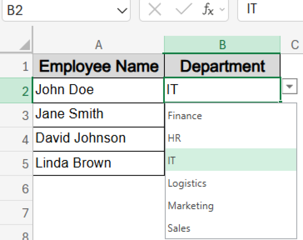
You should now see a small dropdown arrow next to your selected cell. Clicking it will reveal the list of items from your source data range.

Using VLOOKUP to Pull Data Automatically

Once the drop-down list is functional, the next step is to use the VLOOKUP function to automatically retrieve related information from your source sheet based on the selection made in the drop-down list. This is where the magic happens, connecting your selection to comprehensive data.

The VLOOKUP function is essential for looking up information in one table and returning related information from another. Its syntax is:

=VLOOKUP(lookup_value, table_array, col_index_num, [range_lookup])

• lookup_value: This is the cell containing your drop-down list. When a user selects an item, this value is passed to VLOOKUP.
• table_array: This is the named range you created earlier (e.g., EmployeeList). It tells VLOOKUP where to search for the data.
• col_index_num: This is the column number within your table_array from which you want to retrieve data. For instance, if your named range starts with employee names in the first column and you want to pull their department from the second column, this would be 2.
• [range_lookup]: This is an optional argument. Use FALSE for an exact match (highly recommended for most cases) or TRUE for an approximate match.

Example:

Imagine you have a list of employees on Sheet2 with their names in column A and their departments in column B. You’ve created a drop-down list for employee names on Sheet1 in cell A2. To automatically display the employee’s department on Sheet1 in cell B2, you would enter the following formula in B2:

=VLOOKUP(A2, EmployeeList, 2, FALSE)

Here, A2 is the cell with the drop-down, EmployeeList is the named range containing names and departments, 2 indicates you want data from the second column (departments), and FALSE ensures an exact match for the employee’s name.

This setup creates a powerful, interactive spreadsheet where selections automatically trigger data retrieval, minimizing errors and maximizing efficiency.

For further details on implementing drop-down lists and data validation in Excel, you can refer to this comprehensive guide: How to Create a Drop-Down List That Pulls Data From Another Worksheet. This resource provides additional insights and advanced techniques to enhance your Excel skills.

This method of using a drop-down list with VLOOKUP is a fundamental technique for anyone looking to build more robust and user-friendly Excel models. By following these steps, you can significantly improve data management within your spreadsheets.