Introduction
Conditional formatting is a powerful feature in Microsoft Excel that helps you visualize data patterns, trends, and outliers by applying specific formatting rules based on cell values. Whether you’re analyzing monthly temperature data, sales figures, or inventory levels, conditional formatting makes it easier to interpret complex datasets at a glance. This guide explores how to apply, customize, and manage conditional formatting rules to enhance your data analysis and reporting in Excel.
Understanding Conditional Formatting
Conditional formatting allows you to automatically format cells based on their values, such as changing cell colors, fonts, or borders. You can apply it to:
- A range of cells (selected or named)
- An Excel table
- A PivotTable report (with some considerations)

Conditional Formatting in PivotTable Reports
While conditional formatting works similarly in ranges, tables, and PivotTables, there are unique considerations for PivotTables:
- Some formats do not work with fields in the Values area (e.g., formatting based on unique or duplicate values).
- Formatting is maintained if you filter, hide, or rearrange fields, as long as the underlying data remains unchanged.
- The scope of formatting can be based on the data hierarchy, determined by visible children (lower levels) of a parent (higher level) in rows or columns.
Note: In a data hierarchy, children do not inherit formatting from parents, and vice versa.
Applying Conditional Formatting
Method 1: Using the Quick Analysis Button
The Quick Analysis button provides a fast way to apply predefined conditional formatting styles.
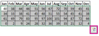
Select the data you want to format. The Quick Analysis button appears at the bottom-right corner of your selection.
 Selected data with the Quick Analysis button
Click the Quick Analysis button (or press Ctrl+Q).
In the Formatting tab, hover over options to preview them in Live Preview, then select your desired format.
 Formatting tab in the Quick Analysis gallery
Note:
- Available options depend on your data type (e.g., Data Bars, Color Scales, Icon Sets for numbers).
- Live Preview only works for compatible formats.
If prompted, enter the formatting criteria (e.g., for Text That Contains) and click OK.
 Selected data with the Quick Analysis button
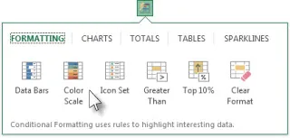 Formatting tab in the Quick Analysis gallery
Method 2: Creating Custom Rules
If the predefined options don’t meet your needs, you can create custom rules:
Select the cells you want to format.
Go to the Home tab > Conditional Formatting > New Rule.
 New formatting rule
Define your rule (e.g., Format cells greater than a value) and specify the format (font, fill, border).
Click OK to apply.
 New formatting rule
Pro Tip: Use formulas for advanced conditions. For example:
=AND(B4<=75000, ABS(B5)<=1500)to format cells where both conditions are met.=MOD(ROW(),2)=1to shade every other row in blue. Every other row is shaded blue
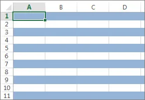 Every other row is shaded blue
Managing Conditional Formatting Rules
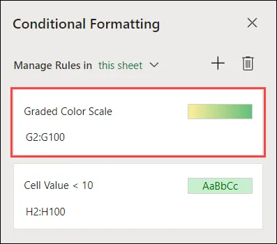
Accessing the Rules Manager
To view, edit, or delete rules:
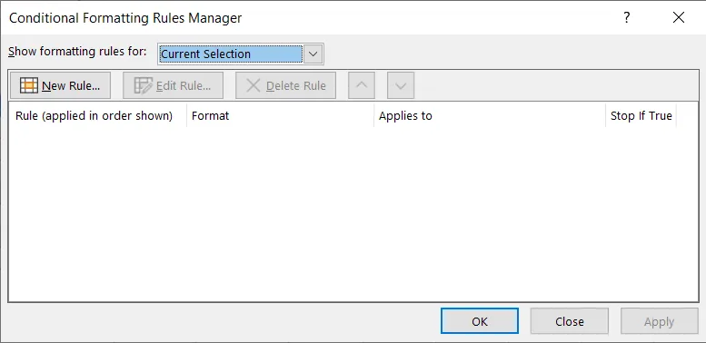
Go to Home > Conditional Formatting > Manage Rules.
The Conditional Formatting Rules Manager dialog box appears.
 Conditional Formatting Rules Manager dialog box
 Conditional Formatting Rules Manager dialog box
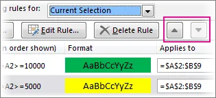
Rule Precedence and Conflicts
Rules are evaluated top to bottom in the Rules Manager.
If multiple rules apply, the highest precedence rule (topmost) takes effect.
Use the Move Up/Down arrows to adjust precedence.
 Move Up and Move Down arrows
 Move Up and Move Down arrows
Example:
- Rule 1: Format cells with expired dates in red.
- Rule 2: Format cells with dates expiring in 60 days in yellow.
- If a cell meets both conditions, Rule 1 (red) applies because it has higher precedence.
Stopping Rule Evaluation
For backward compatibility, use the Stop If True checkbox to mimic older Excel versions (which supported only 3 rules per range). This stops further rules from being evaluated if the current rule is True.
Note: This option is unavailable for rules using data bars, color scales, or icon sets.
Advanced Conditional Formatting Techniques
Using Formulas for Dynamic Rules
Formulas allow you to create highly customized conditions. For example:
- Highlight cells where a product category is “Grain” and sales are below 500:
=AND(B3="Grain", D3<500) - Shade every other row:
=MOD(ROW(),2)=1

Tip: Use relative references (e.g., B3) for dynamic ranges and absolute references (e.g., $B$3) for fixed cells.
Scoping Rules in PivotTables
For PivotTable fields in the Values area, you can scope rules in three ways:
- By selection: Apply to a contiguous or non-contiguous set of fields.
- By value field: Apply to all levels in the hierarchy (including subtotals).
- By corresponding field: Apply to one level in the hierarchy (excluding subtotals).
Use the Apply formatting rule to option in the New/Edit Rule dialog to change scoping.
Clearing Conditional Formatting
To remove conditional formatting:
- From selected cells: Go to Home > Conditional Formatting > Clear Rules > Clear Rules from Selected Cells.
- From the entire sheet: Select Clear Rules from Entire Sheet.
- Delete specific rules: Use the Rules Manager and click the Delete (trash can) icon.
Practical Examples of Conditional Formatting
1. Color Scales
Visualize data distribution using two-color or three-color scales.
Two-color scale: Compare values with a gradient (e.g., green for high, yellow for low).
 Two color scale formatting
Three-color scale: Use three colors (e.g., green, yellow, red) for high, middle, and low values.
 Three color scale formatting
 Two color scale formatting
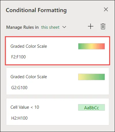 Three color scale formatting
How to apply:
- Select your data range.
- Go to Home > Conditional Formatting > Color Scales and choose a preset.
2. Data Bars
Highlight relative cell values with bars. Longer bars indicate higher values.
How to apply:
- Select your data.
- Go to Home > Conditional Formatting > Data Bars and pick a style.
3. Icon Sets
Classify data into 3–5 categories using icons (e.g., arrows, flags, ratings).
Example: Use 3 Arrows to show:
- Green up arrow: High values
- Yellow sideways arrow: Middle values
- Red down arrow: Low values
How to apply:
- Select your data.
- Go to Home > Conditional Formatting > Icon Sets and choose a set.
4. Highlight Cell Rules
Highlight cells based on specific conditions, such as:
- Greater Than, Less Than, or Between values
- Text That Contains a keyword
- Duplicate Values
Example: Highlight products with stock < 10 to identify restocking needs.
How to apply:
- Select your data.
- Go to Home > Conditional Formatting > Highlight Cell Rules and choose a rule.
5. Top/Bottom Rules
Identify top or bottom performers in a dataset. For example:
- Top 10 items in sales
- Bottom 15% in customer satisfaction
How to apply:
- Select your data.
- Go to Home > Conditional Formatting > Top/Bottom Rules and select an option.
6. Duplicate Values
Quickly spot duplicate entries in your data.
How to apply:
- Select your data.
- Go to Home > Conditional Formatting > Highlight Cell Rules > Duplicate Values.
Copying Conditional Formatting with Format Painter
To copy formatting to other cells:
Select the cell with the desired formatting.
Click Home > Format Painter (the pointer turns into a paintbrush).
Drag the paintbrush over the target cells.
Press Esc to exit.
Note: Adjust cell references in formulas if needed after pasting.
Finding Cells with Conditional Formatting
To locate cells with conditional formatting:
- Click any cell without conditional formatting.
- Go to Home > Find & Select > Conditional Formatting.
To find cells with the same formatting:
- Click a cell with the desired formatting.
- Go to Home > Find & Select > Go To Special > Conditional Formats > Same.
Best Practices for Conditional Formatting
- Keep it simple: Avoid overusing too many rules or colors, as it can make data harder to interpret.
- Use consistent colors: Stick to a color scheme (e.g., green for positive, red for negative).
- Test your rules: Ensure formatting applies correctly by previewing changes.
- Document your rules: Add comments or notes to explain complex formulas.
- Optimize for performance: Large datasets with many rules may slow down Excel. Use efficient formulas and limit the range where possible.
Troubleshooting Common Issues
| Issue | Solution |
|---|---|
| Formatting not applying | Check if the rule’s condition is met. Use ISERROR or IFERROR to handle errors in formulas. |
| Rules conflicting | Adjust precedence in the Rules Manager. |
| Formatting lost after copying | Ensure relative/absolute references are correct. |
| PivotTable formatting not working | Verify the scope (by selection, value field, or corresponding field). |
| Performance lag | Reduce the number of rules or limit the range. |
Conclusion
Conditional formatting is an indispensable tool for anyone working with data in Excel. By mastering its features—from Quick Analysis to custom formulas—you can transform raw data into insightful, visually compelling reports. Whether you’re highlighting trends, identifying outliers, or categorizing data, conditional formatting helps you work smarter, not harder.
Start experimenting with these techniques in your next Excel project and unlock the full potential of your data!
Need more help?
- Ask an expert in the Excel Tech Community.
- Explore Excel for the web for free.