In the realm of measurement system analysis, the ANOVA (Analysis of Variance) method for Gage Repeatability and Reproducibility (R&R) studies stands as a powerful statistical tool. Unlike the traditional average and range method, ANOVA leverages variance analysis to dissect the results of a Gage R&R study, offering deeper insights into the sources of variation. While both methods often yield similar outcomes, ANOVA provides a more robust framework for understanding the nuances of measurement systems.
This article, the first in a multi-part series, delves into the ANOVA table—specifically, the sum of squares and degrees of freedom—and how they are calculated for a Gage R&R study. These concepts are foundational for interpreting the variability in measurement processes, ensuring accuracy, and improving system reliability.
The Importance of Variation in Gage R&R Studies
A Gage R&R study is fundamentally a study of variation. Without variation in the results, the study cannot provide meaningful insights. Occasionally, practitioners may encounter a scenario where all measurements are identical across parts and operators. While consistency might seem desirable, in the context of a Gage R&R study, the absence of variation indicates that the measurement process cannot distinguish between different samples. Thus, variation is not just expected—it is essential.
For those unfamiliar with conducting a Gage R&R study, refer to our guide on variable measurement systems and the average and range method for a comprehensive overview.
Sources of Variation in Measurement Processes
When monitoring a process by measuring a critical quality characteristic (X), the results will naturally vary. This variation stems from multiple sources, which can be categorized into three primary components:
- Process Variation (σₚ²): Inherently tied to the production process itself.
- Sampling Variation (σₛ²): Arises from the method of selecting samples.
- Measurement System Variation (σₘₛ²): Introduced by the measurement tools and procedures.
These components are interrelated through the following equation:
σₜ² = σₚ² + σₛ² + σₘₛ²
Here, σₜ² represents the total process variance, while σₚ², σₛ², and σₘₛ² denote the variances due to the process, sampling, and measurement system, respectively. For simplicity, we often consolidate sampling variation into the process variance, simplifying the equation to:
σₜ² = σₚ² + σₘₛ²
This relationship can be visualized using a right triangle, where:
- The hypotenuse represents the total standard deviation (σₜ).
- One leg represents the process standard deviation (σₚ).
- The other leg represents the measurement system standard deviation (σₘₛ).
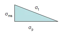
This geometric representation highlights how changes in product variation and measurement system variation impact the total variation. If the measurement system variation (σₘₛ) becomes too large, it can dominate the total variation, undermining the reliability of the measurement process. Therefore, the primary objective in improving a measurement system is to minimize the percentage of variance attributed to the measurement system:
% Variance due to Measurement System = 100 × (σₘₛ² / σₜ²)
Breaking Down Measurement System Variation
In a Gage R&R study, the measurement system variation (σₘₛ²) can be further decomposed into two critical components:
Repeatability:
This refers to the ability of the measurement system to produce identical results when the same operator measures the same part under the same conditions. It assesses the consistency of measurements for a single operator and part combination.Reproducibility:
This evaluates the consistency of measurements across different operators, parts, or conditions. It reflects the ability of the measurement system to yield the same results when different operators measure the same part.
The ANOVA method provides a systematic approach to quantifying both repeatability and reproducibility, thereby offering a comprehensive understanding of the measurement system’s performance.
Example Data for Gage R&R Study
To illustrate the calculations, we will use data from a previous study on the average and range method for Gage R&R. In this example:
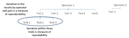
- 3 operators tested 5 parts, with 3 trials per part.
- The layout of the study is depicted below:
Understanding the Sources of Variation
Within Variation (Repeatability):
For a single operator measuring the same part multiple times (e.g., Operator 1 testing Part 1 three times), the variation in results is attributed solely to the measurement equipment. This is also known as equipment variation or within variation in ANOVA studies.Between Variation (Reproducibility):
When operators test different parts, the variation includes contributions from the parts themselves, the operators, and the interaction between operators and parts. This cumulative variation is referred to as reproducibility.
The data from the study is presented in the table below:
Gage R&R Study Data: Measurement Results by Operator and Part
| Operator | Part | Trial 1 | Trial 2 | Trial 3 |
|---|---|---|---|---|
| A | 1 | 3.29 | 3.41 | 3.64 |
| A | 2 | 2.44 | 2.32 | 2.42 |
| A | 3 | 4.34 | 4.17 | 4.27 |
| A | 4 | 3.47 | 3.50 | 3.64 |
| A | 5 | 2.20 | 2.08 | 2.16 |
| B | 1 | 3.08 | 3.25 | 3.07 |
| B | 2 | 2.53 | 1.78 | 2.32 |
| B | 3 | 4.19 | 3.94 | 4.34 |
| B | 4 | 3.01 | 4.03 | 3.20 |
| B | 5 | 2.44 | 1.80 | 1.72 |
| C | 1 | 3.04 | 2.89 | 2.85 |
| C | 2 | 1.62 | 1.87 | 2.04 |
| C | 3 | 3.88 | 4.09 | 3.67 |
| C | 4 | 3.14 | 3.20 | 3.11 |
| C | 5 | 1.54 | 1.93 | 1.55 |
The ANOVA Table for Gage R&R
In practice, software tools (e.g., SPC for Excel) are typically used to perform the calculations for a Gage R&R study. However, understanding the manual calculations enhances comprehension of the underlying principles. The results are typically presented in an ANOVA table, which includes the following columns:
- Source of Variability: Identifies the factor contributing to variation (e.g., operator, part, interaction, equipment).
- Degrees of Freedom (df): The number of independent values that can vary in the analysis.
- Sum of Squares (SS): A measure of variation for each source, calculated as the sum of squared deviations from the mean.
- Mean Square (MS): The sum of squares divided by the degrees of freedom, providing an estimate of the variance for each source.
- F Value: A test statistic used to determine the statistical significance of each source of variability.
- p Value: The probability that the observed variation is due to random chance.
The ANOVA table for our example data is shown below:
ANOVA Table for Gage R&R Study
| Source | df | SS | MS | F | p Value |
|---|---|---|---|---|---|
| Operator | 2 | 1.630 | 0.815 | 100.322 | 0.0000 |
| Part | 4 | 28.909 | 7.227 | 889.458 | 0.0000 |
| Operator × Part | 8 | 0.065 | 0.008 | 0.142 | 0.9964 |
| Equipment | 30 | 1.712 | 0.057 | – | – |
| Total | 44 | 32.317 | – | – | – |
Calculating the Sum of Squares and Degrees of Freedom
1. Total Sum of Squares (SST) and Degrees of Freedom
The total sum of squares (SST) is the sum of the squared deviations of each individual result from the overall average (the mean of all 45 results). Mathematically, it is expressed as:
where Xᵢⱼₘ represents the result for the i-th operator, j-th part, and m-th trial.
For our dataset, the overall average is calculated as 2.9867. The SST is then computed as 32.317, with the calculations detailed in the table below:
Calculations for Total Sum of Squares (SST)
| Operator | Part | Trial 1 | Trial 2 | Trial 3 | Squared Deviation (Trial 1) | Squared Deviation (Trial 2) | Squared Deviation (Trial 3) |
|---|---|---|---|---|---|---|---|
| A | 1 | 3.29 | 3.41 | 3.64 | 0.120 | 0.217 | 0.485 |
| A | 2 | 2.44 | 2.32 | 2.42 | 0.254 | 0.389 | 0.274 |
| A | 3 | 4.34 | 4.17 | 4.27 | 1.949 | 1.504 | 1.759 |
| A | 4 | 3.47 | 3.50 | 3.64 | 0.277 | 0.309 | 0.485 |
| A | 5 | 2.20 | 2.08 | 2.16 | 0.553 | 0.746 | 0.614 |
| B | 1 | 3.08 | 3.25 | 3.07 | 0.019 | 0.094 | 0.016 |
| B | 2 | 2.53 | 1.78 | 2.32 | 0.171 | 1.354 | 0.389 |
| B | 3 | 4.19 | 3.94 | 4.34 | 1.553 | 0.992 | 1.949 |
| B | 4 | 3.01 | 4.03 | 3.20 | 0.004 | 1.180 | 0.066 |
| B | 5 | 2.44 | 1.80 | 1.72 | 0.254 | 1.308 | 1.498 |
| C | 1 | 3.04 | 2.89 | 2.85 | 0.009 | 0.003 | 0.009 |
| C | 2 | 1.62 | 1.87 | 2.04 | 1.752 | 1.153 | 0.817 |
| C | 3 | 3.88 | 4.09 | 3.67 | 0.877 | 1.314 | 0.527 |
| C | 4 | 3.14 | 3.20 | 3.11 | 0.039 | 0.066 | 0.028 |
| C | 5 | 1.54 | 1.93 | 1.55 | 1.971 | 1.028 |
The degrees of freedom (df) for the total sum of squares is 44 (45 results – 1).
2. Operator Sum of Squares (SSO) and Degrees of Freedom
The operator sum of squares (SSO) measures the squared deviations of each operator’s average from the overall average. The formula is:
where n is the number of parts (5), r is the number of trials (3), and nr is the number of results per operator (15).
The calculations for SSO are summarized in the table below:
Calculations for Operator Sum of Squares (SSO)
| Operator | Operator Average | Squared Deviation for Operator |
|---|---|---|
| A | 3.1567 | 0.0453 |
| B | 2.9800 | 0.0013 |
| C | 2.6947 | 0.0621 |
| Sum of Deviations | – | 0.1087 |
| 15 × (Sum of Deviations) | – | 1.6304 |
Thus, SSO = 1.6304.
The degrees of freedom for operators is 2 (3 operators – 1).
3. Parts Sum of Squares (SSP) and Degrees of Freedom
The parts sum of squares (SSP) is calculated similarly to the operator sum of squares, but it focuses on the deviations of part averages from the overall average. The formula is:
where k is the number of operators (3), r is the number of trials (3), and kr is the number of results per part (9).
The calculations for SSP are detailed in the table below:
Calculations for Parts Sum of Squares (SSP)
| Part | Part Average | Squared Deviation for Part |
|---|---|---|
| 1 | 3.1689 | 0.0507 |
| 2 | 2.1489 | 0.6318 |
| 3 | 4.0989 | 1.3343 |
| 4 | 3.3667 | 0.1788 |
| 5 | 1.9356 | 1.0165 |
| Sum of Deviations | – | 3.2122 |
| 9 × (Sum of Deviations) | – | 28.9094 |
Thus, SSP = 28.9094.
The degrees of freedom for parts is 4 (5 parts – 1).
4. Equipment (Within) Sum of Squares (SSE) and Degrees of Freedom
The equipment sum of squares (SSE) measures the variation within the three trials for each operator-part combination. It is calculated as the sum of squared deviations of each trial from the average of the three trials for that operator and part. The formula is:
The calculations for SSE are shown in the table below:
Calculations for Equipment (Within) Sum of Squares (SSE)
| Operator | Part | Trial 1 | Trial 2 | Trial 3 | Average of 3 Trials | Squared Deviation (Trial 1) | Squared Deviation (Trial 2) | Squared Deviation (Trial 3) |
|---|---|---|---|---|---|---|---|---|
| A | 1 | 3.29 | 3.41 | 3.64 | 3.447 | 0.025 | 0.001 | 0.037 |
| A | 2 | 2.44 | 2.32 | 2.42 | 2.393 | 0.002 | 0.005 | 0.001 |
| A | 3 | 4.34 | 4.17 | 4.27 | 4.260 | 0.006 | 0.008 | 0.000 |
| A | 4 | 3.47 | 3.50 | 3.64 | 3.537 | 0.004 | 0.001 | 0.011 |
| A | 5 | 2.20 | 2.08 | 2.16 | 2.147 | 0.003 | 0.004 |
Thus, SSE = 1.712.
The degrees of freedom for equipment variation is 30 (nk(r-1) = 3 operators × 5 parts × (3 trials – 1)).
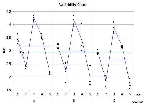
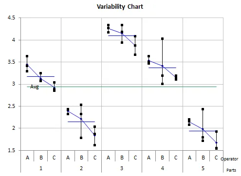 Variability chart by part, showing results for each operator-part combination
5. Interaction Sum of Squares (SSO×P) and Degrees of Freedom
The interaction sum of squares (SSO×P) is derived from the relationship:
SST = SSO + SSP + SSO×P + SSE
Rearranging the equation to solve for SSO×P:
SSO×P = SST – (SSO + SSP + SSE)
SSO×P = 32.317 – (1.630 + 28.909 + 1.712) = 0.065
Similarly, the degrees of freedom for interaction is calculated as:
dfO×P = dfT – (dfO + dfP + dfE)
dfO×P = 44 – (2 + 4 + 30) = 8
Summary and Next Steps
This article provided a detailed explanation of how the sum of squares and degrees of freedom are calculated for an ANOVA-based Gage R&R study. These foundational concepts are critical for understanding the sources of variation in measurement systems and ensuring the reliability of your processes.
In the next installment of this series, we will complete the ANOVA table and finalize the Gage R&R calculations, including the estimation of repeatability, reproducibility, and total measurement system variation. Stay tuned for a deeper dive into the practical applications of ANOVA in measurement system analysis!